An Introduction to Ibis for Python Programmers
A More Pythonic Way To Work With Databases
A few weeks ago I was working on setting up a relational database to explore records from DataSF’s Civic Art Collection. Whenever I attend a tech conference I try to spend a day or two in the city to check out it’s cultural scene, so this seemed like useful information! I decided to use MySQL as my database engine. Coming from a Pandas background I was surprised by how unproductive and restricted I felt writing raw SQL queries. I also spent a significant amount of time resolving errors in queries that worked with one flavor of SQL but failed with MySQL. Throughout the process I kept thinking to myself if only there was a more Pythonic way!!! A few weeks later I was introduced to Ibis.
Ibis provides a more Pythonic way of interacting with multiple database engines. In my own adventures I’ve always encountered Ibis’s (the bird versions) perched on top of elephants. If you’ve never seen an elephant in real life I can confirm that they are huge, complex creatures. Here’s a picture of me standing next to some for scale ;)

The image of a small bird sitting on top of a large elephant serves as a metaphor for how ibis provides a less complex, more performant way for users to interact with multiple big data engines. In fact the bigger and more complex your data the more of an argument there is to use Ibis. SQL can be quite difficult to maintain when your queries are very complex. With ibis there is no need to completely rewrite your code whether you’re scaling up or down. You can switch out your back-end if you need to and keep working in the same context but with a more powerful engine. This means your workflow is streamlined, less error prone and your cognitive load is reduced.
At the moment, Ibis supports quite a few backends including:
Traditional DBMSs: PostgreSQL, MySQL, SQLite Analytical DBMSs: OmniSciDB, ClickHouse, Datafusion Distributed DBMSs: Impala, PySpark, BigQuery In memory analytics: pandas, Dask
Whether you’re wanting to interact with SQL databases or wanting to use distributed DBMSs, Ibis lets you do this in Python. In this post I’ll be using an SQLite backend but if you’d like to try any of the others checkout the Ibis backends page for examples. Ibis currently supports over 12 backends, some of which compile to SQL and some of which are directly executed.
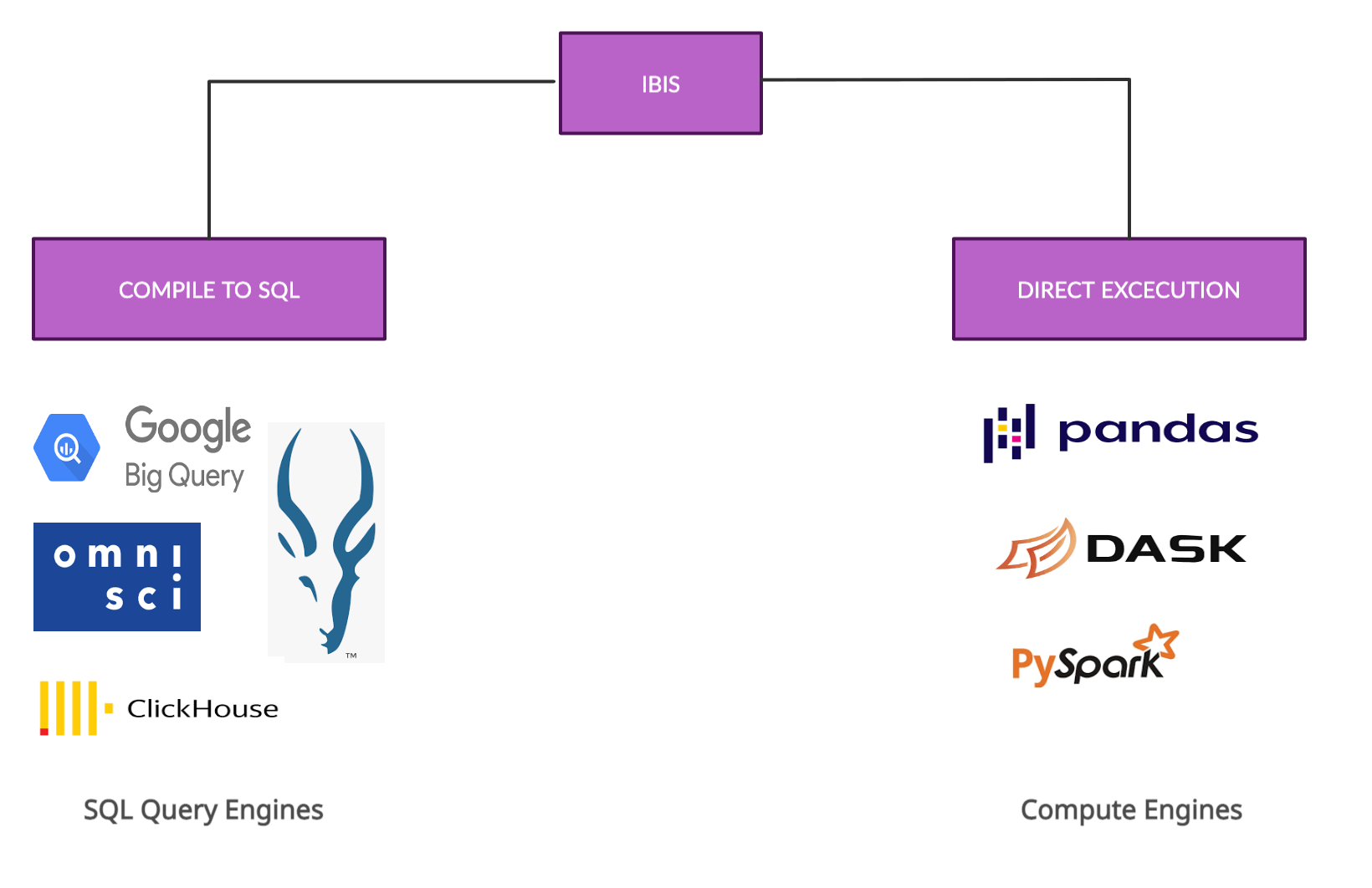
For Python programmers Ibis offers a way to write SQL in Python that allows for unit-testing, composability, and abstraction over specific query engines (e.g.BigQuery)! You can carry out joins, filters and other operations on your data in a familiar, Pandas-like syntax. Overall, using Ibis simplifies your workflows, makes you more productive, and keeps your code readable.
Let’s use the Civic Art Collection dataset I mentioned earlier and see what Ibis can do!
Installation
You can install Ibis with Pip, Conda or Mamba.
For the sake of security, I’d recommend setting up a virtual environment. You can copy and paste these commands into your terminal to install ibis with either Pip or Conda.
Pip:
In this tutorial we’ll be using SQLite as our backend. If you use pip to install Ibis you’ll need to run pip install 'ibis-framework[sqlite]' instead of the usual pip install ibis-framework for sqlite to work. If you’d prefer to use another backend look for the specific commands in the Ibis documentation.
Mac:
python3 -m venv ibisdev
source ibisdev/bin/activate
pip install 'ibis-framework[sqlite]'
pip install pysqlite
Windows:
python3 -m venv ibisdev
ibisdev\Scripts\activate.bat
pip install 'ibis-framework[sqlite]'
pip install pysqlite
Conda
conda create -n ibisdev python=3.8
conda activate ibisdev
conda install -c conda-forge ibis-framework
conda install -c anaconda sqlite
Creating a database with SQLite
If you’d like to follow along with me, the next thing we’ll do is create a database and a table containing data about art around San Francisco from DataSF. The data is open source so you can download the csv file directly from the site. Ibis doesn’t support loading csv files into an SQL table yet, so we’ll follow these commands to do so in the command line with SQLite
Create a folder called civic_art
mkdir civic_art
cd civic_art
To make things easier in the next steps, I moved the csv file from my downloads folder into the civic_art folder we just created. While we’re in the civic_art folder we create a new database with the following command.
Create a database named civicArt.db
sqlite3 civicArt.db
This command should also open SQLite in your command line. Here’s a picture of what this looks like for me (I used .databases to double check that the database was correctly created.)

Great! The database has successfully been created! SQLite opens up already in the civicArt database so the next thing we’ll do is create a table and load the data from the csv file into it.
Create a table in the civicArt.db database called civicArtTable
.mode csv civicArtTable (names the table)
.import Civic_Art_Collection.csv civicArtTable (import the data into the table)
Check that the table has been created as expected
.tables   (this lets you check the table has been correctly created)
.schema civicArtTable (describes the table)
If your table has been created as expected you can now exit SQLite by typing in .quit. This should take you back to your command line. We’re now ready to start exploring our data with ibis!
Connecting to the database
One of the advantages of ibis is that it lets you work with tools you’re most comfortable with. I enjoy writing Python code in IPython, but you can use a jupyter notebook or any Python shell you’d like. Whatever you choose we'll use the same commands to connect to the civicArt database we created earlier.
Connecting to our database (we’ll be using Ibis’ interactive mode for lazy evaluation)
import ibis
ibis.options.interactive = True
db = ibis.sqlite.connect("civicArt.db")
Something to note here is that pandas (read_sql) loads data into memory and performs the computations itself. Ibis won't load the data or perform any computation. Instead it leaves the data in the database defined by the connection, and will ask the backend to perform the computations there. This means you can execute at the speed of your backend, not your local computer. A good way to think about this is to go back to our elephant metaphor. If you need some heavy lifting done, it’s probably a good idea to let an elephant do it as compared to an ibis. Our elegant ibis can pass on the heavier work to the larger database and watch as the work is done much faster than it could have done itself.

If everything went well you should be connected to the database. We’ll take a look at our data next!
Viewing Table Details
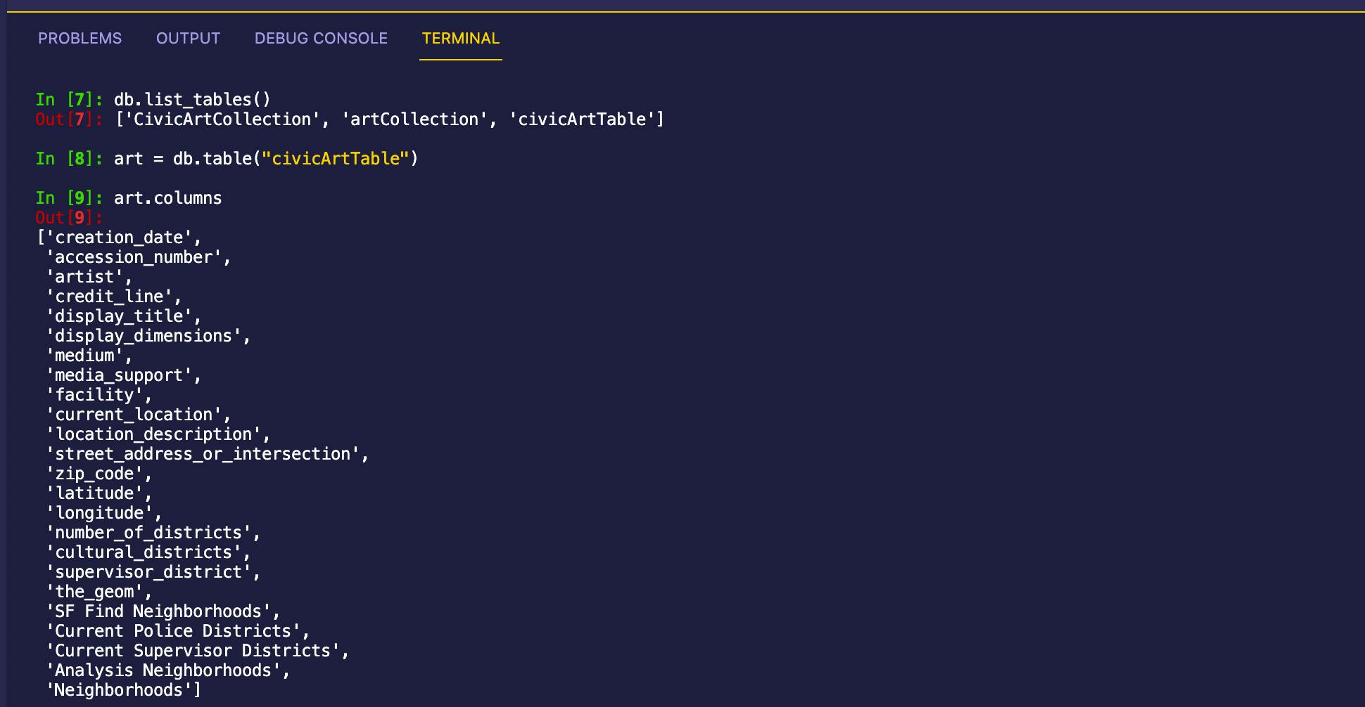
Let's use Ibis to take a look at the tables in the civicArt database
List out all the tables in the database
db.list_tables()
Assign the table to a more readable name and list the columns in it
art = db.table("civicArtTable")
art.columns
This is what I’m seeing in IPython after calling these commands
Wrangling Data With Ibis
Let's now use Ibis to carry out some common SQL commands on our dataset and find out some useful information about art in San Francisco in the process.
Querying
Anything you can write in a SELECT statement you can write in Ibis. Let's test this out! I’ll use the following code to find out which artists have art currently displayed in the city and what the title of their pieces are.
Selecting columns from a table
art["artist", "display_title"]
Great! If you’ve used Pandas before this should feel similar to getting columns from a Pandas Dataframe, but remember the database is doing all the work for us, so this is more efficient!

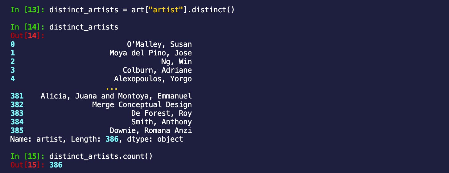
I’m also curious about how many artists total have their work on display in case an artist has more than one piece exhibited. To do this let's get distinct artists and then count them
Distinct and Count
distinct_artists = art["artist"].distinct()
distinct_artists.count()
We can already see the length of the list, but just to show you the count method, we confirm that the number of artists that have one or more pieces on display in San Francisco is 386!
Filtering Data
Next let's pick an artist and figure out where exactly all their art is located. Adriane Colburns’ display title, Geological Ghost caught my eye so let's choose them!
I use the following commands to do this
adrianes_art = art.filter(art["artist"] == 'Colburn, Adriane')
adrianes_art

So it turns out Adriane has two pieces on display, one at 4 Guy Place and the other at Dagget Street & 16th Street. This is great, we already have some places we can add to our tourist itinerary!
Groupby
I don’t usually stay more than one or two days in a city after a conference, so it might be nice to know which locations have the most art on display. To figure this out we’ll use the following groupby expressions to get the information we need.
Use groupy and sort_by to get locations in San Francisco with the most art!
art_loc = art.groupby("street_address_or_intersection").count('display_title')
most_art = art_loc.sort_by(ibis.desc(art_loc.display_title))
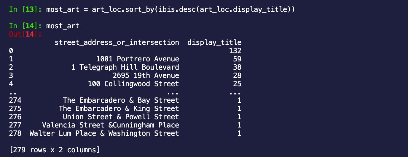
Great, the first stop would be 1001 Potrero Avenue which has 59 titles on display!!
Out of curiosity, I searched 1001 Potrero Avenue to learn more about what I expected would be an art gallery. Surprisingly it turned out to be the Zuckerberg San Francisco General Hospital. They’ve apparently invested a lot in art and have an incredible collection. The thing with data is that it can surprise you! The next best option is Coit tower which has its address at 1 Telegraph Hill Blvd. It is not a hospital and looks like a great place to explore!

credit: Janice Heckert
Joins
Excellent. At this point we know that the next time we’re in San Francisco for a tech conference we have some great options to check out. I only found out after writing my code so let's imagine 1001 Potrero Avenue is not a hospital and use it as our first choice! Now we know where to go. What's next?
Well, oftentimes art galleries are filled with hipsters that will likely ask you about the artists on display. The good thing is that we can prepare for this in advance! Lets use an inner join to help us find which artists have the most art showing so we can look them up and feel cool by having a good response ;)
Use inner_join to find the most popular artists
artist_location = art["street_address_or_intersection", "artist"]
artists_at_portrero = artist_location.filter(artist_location["street_address_or_intersection"] == "1001 Portrero Avenue").distinct()
*ibis version 2.1.1 sometimes encounters an issue with views note being materialized and then materialize not resolving column names on a join operation. The following code fragment is just for version 2.1.1 and uses the mutate() function (first line) to change one of the column headers and materialize() to ensure that the created view can be displayed. This should be fixed in version 3.0.0.
artist_number_of_displays = art.mutate(c_artist=art['artist']).groupby("c_artist").count("display_title")

most_popular_artist = artists_at_portrero.inner_join(
    artist_number_of_displays,
    predicates=artists_at_portrero["artist"] == artist_number_of_displays["c_artist"]
    ).materialize()
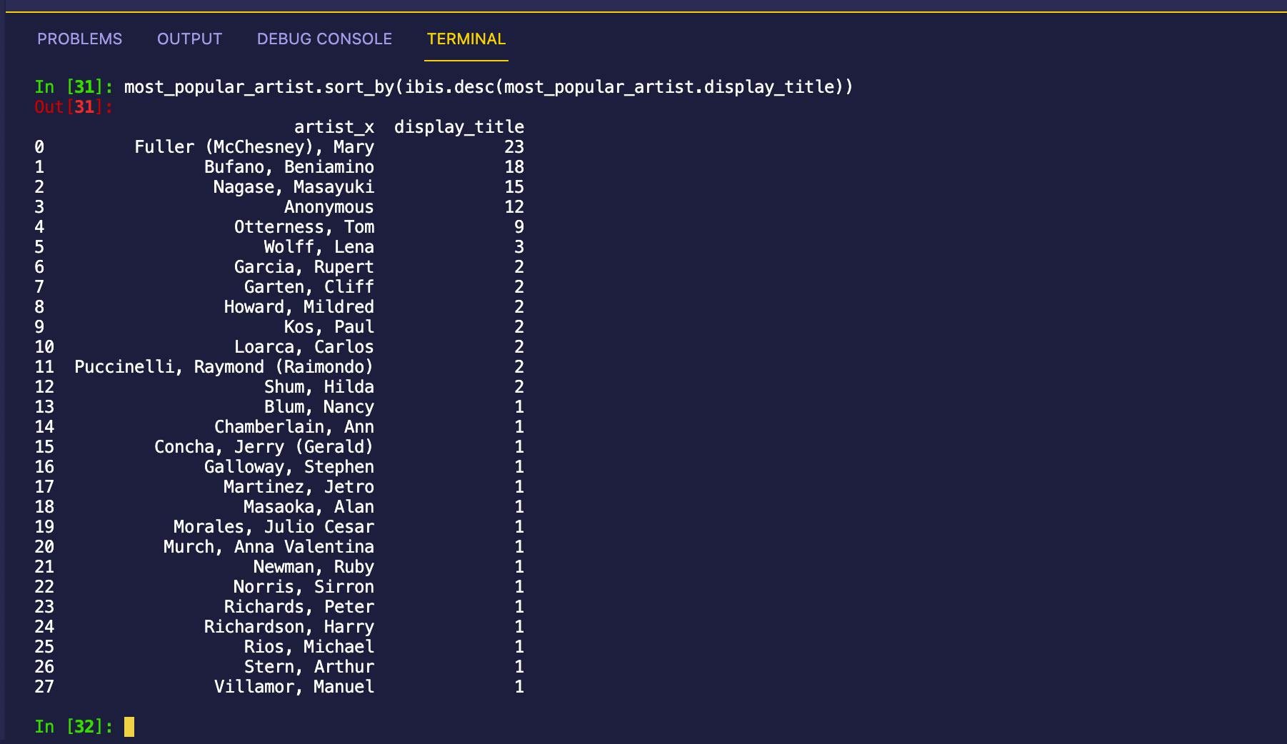
Fantastic! We now know Mary (McChesney) Fuller has the most art on display at 1001 Potrero Avenue and can search online to find out more! In my opinion, we’re as ready as we’ll ever be to explore the art scene in SF!
We learned a lot of information in a relatively short amount of time. If you’re used to writing Python code this probably feels more efficient than writing out raw SQL strings. It also means if you started your workflow in IPython or a Jupyter Notebook you can stay there. This should feel smoother and hopefully lead to increased productivity. Using tools that help you be more efficient means you have more time for creativity and exploration in your work! I wish this for you! Thanks for reading and hopefully I’ll bump into you watching elephants or in an art gallery somewhere around the world!
We've also made a jupyter notebook that has all of the commands in this post! You can find it here
